Get started with ccsgp!
- Authors
- Patrick Huck (GitHub),
original
default_colorsinccsgp_get_started.ccsgp.configcontributed by Johanna Huck - Date
- February 06, 2016
get started with the ccsgp plotting library
Examples Module
The examples are based on a dataset of World Bank Indicators. You can use the
dataset yourself to play around [1]. See the genExDat.sh script in the
same directory on how I extracted the data into the correct format for ccsgp.
To generate all example plots based on ccsgp_get_started_data you can run:
$ python -m ccsgp_get_started
| [1] | ccsgp_get_started_data/input/examples/gp_datdir/{WorldBankIndicators.csv, genExDat.sh} |
Alternatively, you can run a specific module, for instance:
$ python -m ccsgp_get_started.examples.gp_datdir [--log] <country-initial> <#-most-populated>
and this way plot specific country initials. You can open all resulting pictures
via $ open examplesDir/examples/gp_datdir/*.pdf or use pdfnup to put
multiple plots on one page. To start on your own read the documentation below or
the source code and use one of the examples as a template.
-
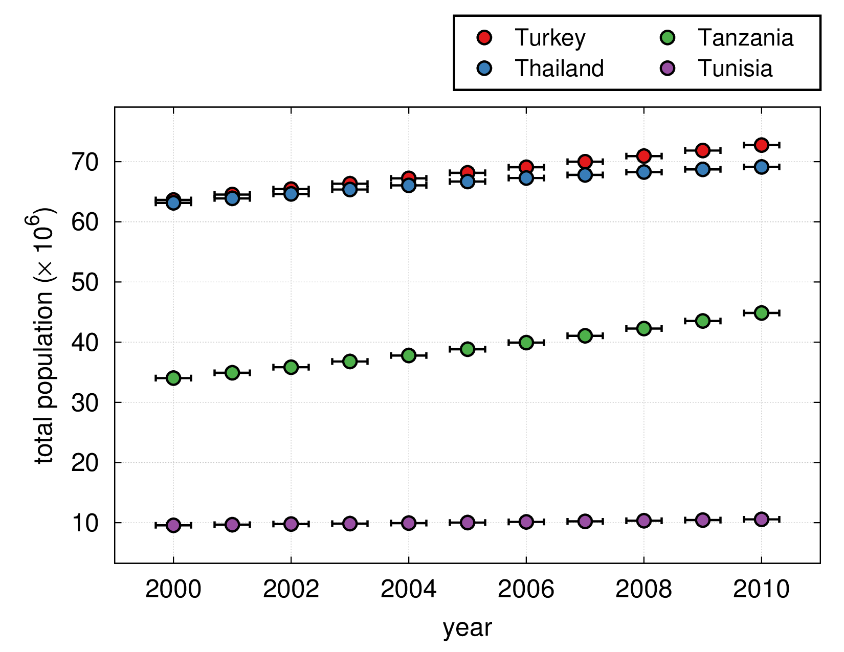
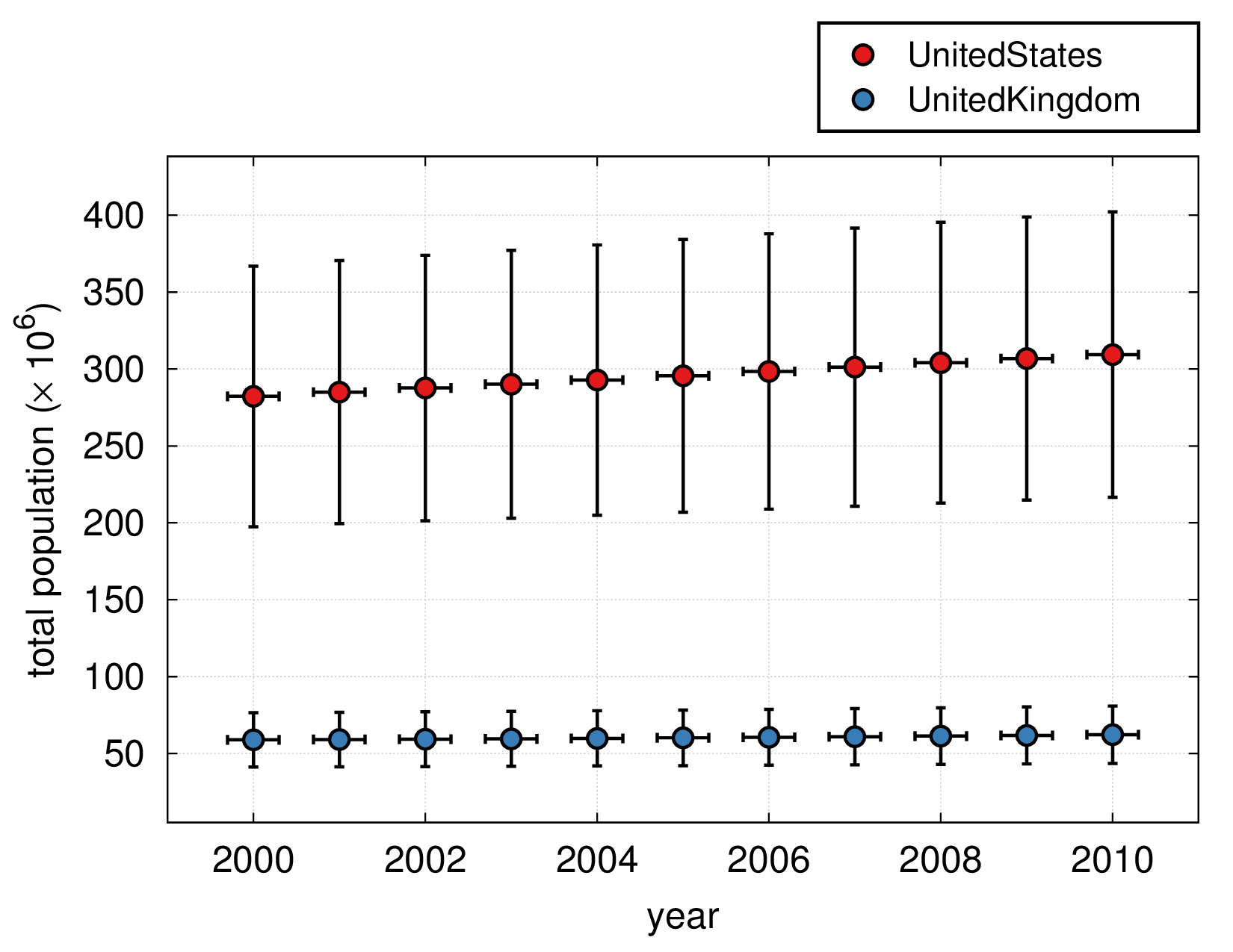
ccsgp_get_started.examples.gp_datdir.gp_datdir(initial, topN)[source]¶ example for plotting from a text file via numpy.loadtxt
- prepare input/output directories
- load the data into an OrderedDict() [adjust axes units]
- sort countries from highest to lowest population
- select the <topN> most populated countries
- call ccsgp.make_plot with data from 4
Below is an output image for country initial T and the 4 most populated countries for this initial (click to enlarge). Also see:
$ python -m ccsgp_get_started.examples.gp_datdir -h
for help on the command line options.
Parameters: Variables: - inDir – input directory according to package structure and initial
- outDir – output directory according to package structure
- data – OrderedDict with datasets to plot as separate keys
- file – data input file for specific country, format: [x y] OR [x y dx dy]
- country – country, filename stem of input file
- file_url – absolute url to input file
- nSets – number of datasets
-
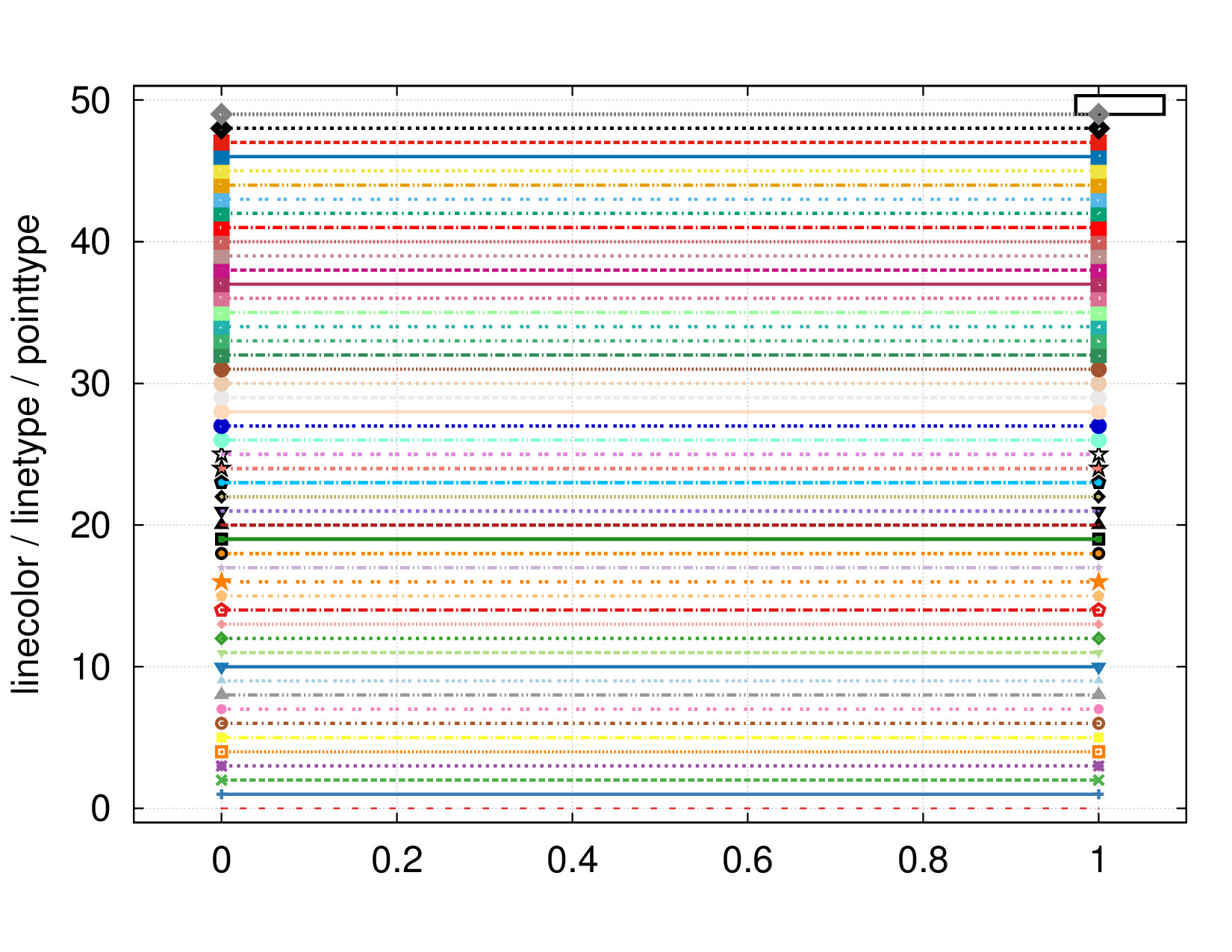
ccsgp_get_started.examples.gp_lcltpt.gp_lcltpt()[source]¶ example plot to display linecolors, linetypes and pointtypes
-
ccsgp_get_started.examples.gp_xfac.gp_xfac()[source]¶ example using QM12 enhancement factors
- uses gpcalls kwarg to reset xtics
- numpy.loadtxt needs reshaping for input files w/ only one datapoint
- according poster presentations see QM12 & NSD review
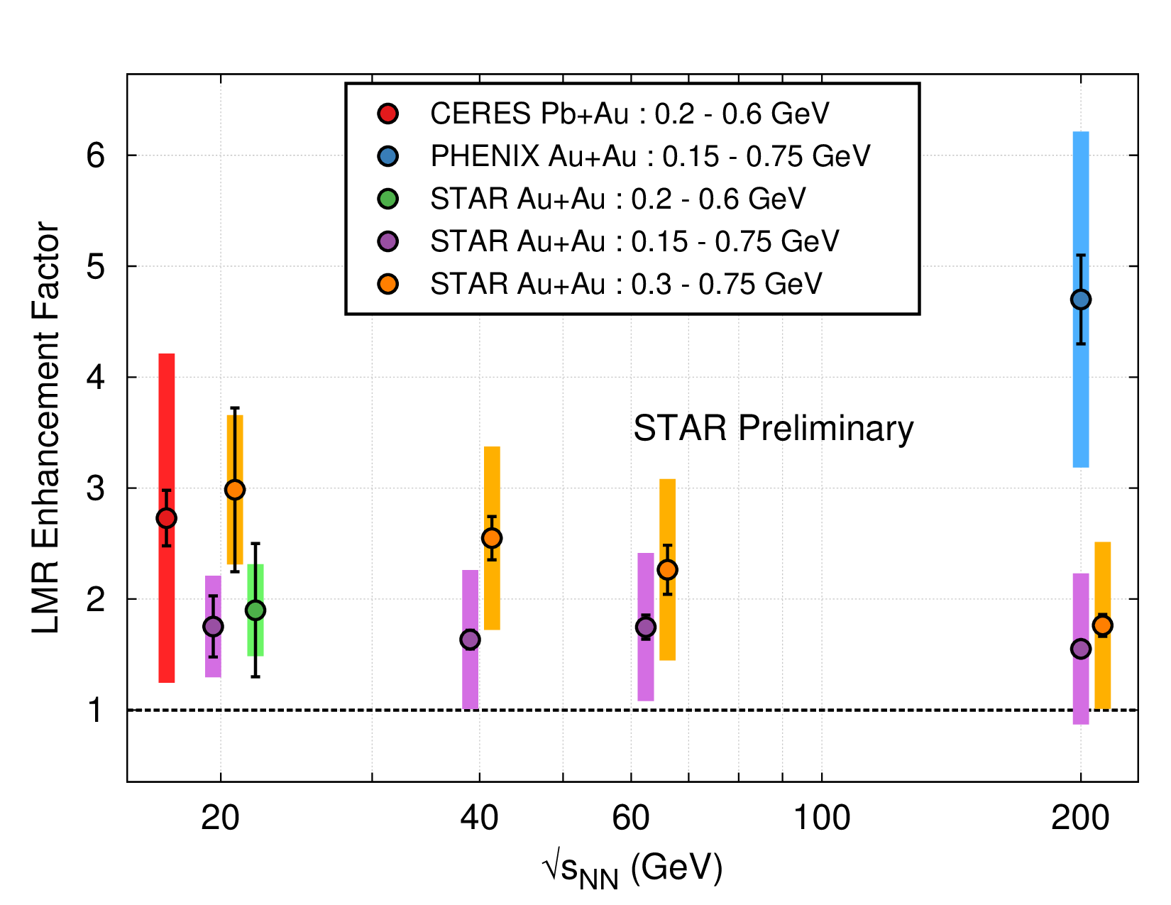
Variables: - key – translates filename into legend/key label
- shift – slightly shift selected data points
-
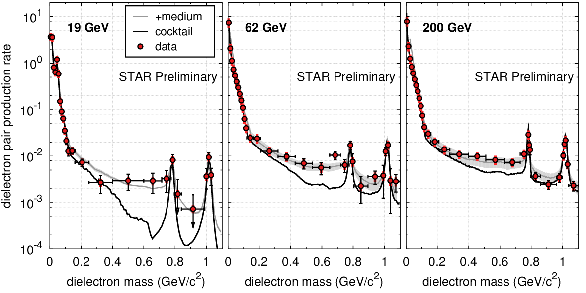
ccsgp_get_started.examples.gp_panel.gp_panel(version, skip)[source]¶ example for a panel plot using QM12 data (see gp_xfac)
Parameters: version (str) – plot version / input subdir name
-
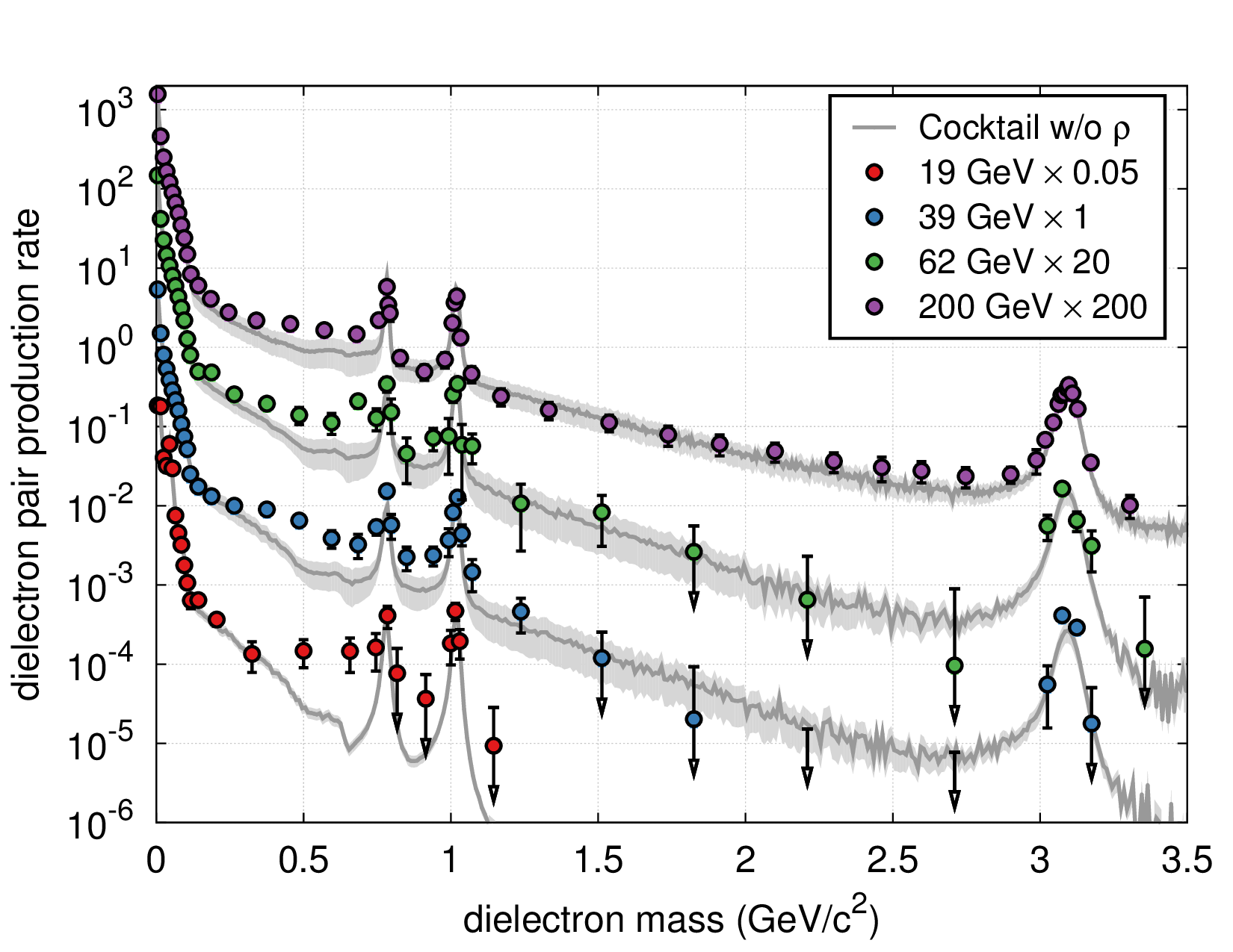
ccsgp_get_started.examples.gp_stack.gp_stack(version, energies, inclMed, inclFits)[source]¶ example for a plot w/ stacked graphs using QM12 data (see gp_panel)
- how to omit keys from the legend
- manually add legend entries
- automatically plot arrows for error bars larger than data point value
Parameters: version (str) – plot version / input subdir name
-
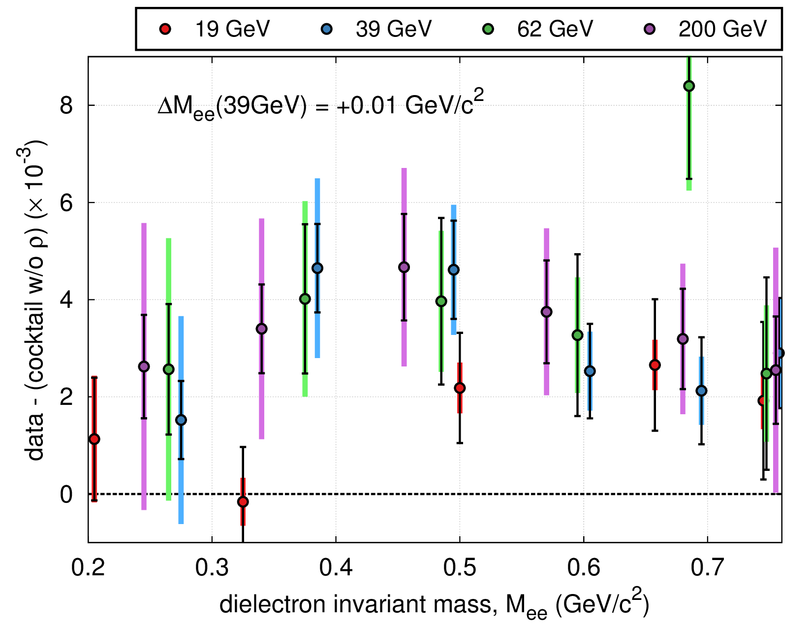
ccsgp_get_started.examples.gp_rdiff.gp_rdiff(version, nomed, noxerr, diffRel, divdNdy)[source]¶ example for ratio or difference plots using QM12 data (see gp_panel)
- uses uncertainties package for easier error propagation and rebinning
- stat. error for medium = 0!
- stat. error for cocktail ~ 0!
- statistical error bar on data stays the same for diff
- TODO: implement ratio!
- TODO: adjust statistical error on data for ratio!
- TODO: adjust name and ylabel for ratio
Parameters:
-
ccsgp_get_started.examples.utils.enumzipEdges(eArr)[source]¶ zip and enumerate edges into pairs of lower and upper limits
-
ccsgp_get_started.examples.utils.getCocktailSum(e0, e1, eCocktail, uCocktail)[source]¶ get the cocktail sum for a given data bin range
-
ccsgp_get_started.examples.utils.getErrorComponent(result, tag)[source]¶ get total error contribution for component with specific tag
ccsgp
ccsgp is a plotting library based on gnuplot-py which wraps the necessary
calls to gnuplot-py into one function called make_plot. The keyword
arguments to make_plot provide easy control over the plot-by-plot dependent
options while reasonable defaults for legend, grid, borders, font sizes,
terminal etc. are handled internally. By providing the data in a default and
reasonable format, the user does not need to deal with the details of
“gnuplot’ing” nor the internals of the gnuplot-py interface library. Every call
of make_plot dumps an ascii representation of the plot in the terminal and
generates the eps hardcopy original. The eps figure is also converted
automatically into pdf, png and jpg formats for easy inclusion in presentations
and papers. In addition, the user can decide to save the data contained in each
image into hdf5 files for easy access via numpy. The function repeat_plot
allows the user replot a specific graph with different properties, like axis
ranges for instance. The make_panel user function facilitates plotting of
1D- or 2D-panel images with merged axes.
The name ccsgp stands for “Carbon Capture and Sequestration GnuPlot” as this library started off in the context of my wife’s research. I knew how to produce nice-looking plots using gnuplot but wanted to hook it up to python directly. The resulting library let’s me generate identical plots independent of the data input source (ROOT, YAML, txt, pickle, hdf5, ...) using the full power of python.
Gnuplot – A pipe-based interface to the gnuplot plotting program.
This is the main module of the Gnuplot package.
Written by “Michael Haggerty”, mailto:mhagger@alum.mit.edu. Inspired by and partly derived from an earlier version by “Konrad Hinsen”, mailto:hinsen@ibs.ibs.fr. If you find a problem or have a suggestion, please “let me know”, mailto:mhagger@alum.mit.edu. Other feedback would also be appreciated.
The Gnuplot.py home page is at
“Gnuplot.py”, http://gnuplot-py.sourceforge.net
For information about how to use this module:
- Check the README file.
- Look at the example code in demo.py and try running it by typing ‘python demo.py’ or ‘python __init__.py’.
- For more details see the extensive documentation strings throughout the python source files, especially this file, _Gnuplot.py, PlotItems.py, and gp_unix.py.
- The docstrings have also been turned into html which can be read “here”, http://gnuplot-py.sourceforge.net/doc. However, the formatting is not perfect; when in doubt, double-check the docstrings.
You should import this file with ‘import Gnuplot’, not with ‘from Gnuplot import *‘, because the module and the main class have the same name, `Gnuplot’.
To obtain the gnuplot plotting program itself, see “the gnuplot FAQ”, ftp://ftp.gnuplot.vt.edu/pub/gnuplot/faq/index.html. Obviously you need to have gnuplot installed if you want to use Gnuplot.py.
The old command-based interface to gnuplot (previously supported as ‘oldplot.py’) has been removed from the package.
Features:
- o Allows the creation of two or three dimensional plots from
- python.
- o A gnuplot session is an instance of class ‘Gnuplot’. Multiple
sessions can be open at once. For example:
g1 = Gnuplot.Gnuplot()
g2 = Gnuplot.Gnuplot()
Note that due to limitations on those platforms, opening multiple simultaneous sessions on Windows or Macintosh may not work correctly. (Feedback?)
- o The implicitly-generated gnuplot commands can be stored to a file
instead of executed immediately:
g = Gnuplot.Gnuplot('commands.txt')The ‘commands.txt’ file can then be run later with gnuplot’s ‘load’ command. Beware, however: the plot commands may depend on the existence of temporary files, which will probably be deleted before you use the command file.
o Can pass arbitrary commands to the gnuplot command interpreter:
    g('set pointsize 2')

(If this is all you want to do, you might consider using the
lightweight GnuplotProcess class defined in gp.py.)
- o A Gnuplot object knows how to plot objects of type ‘PlotItem’.
Any PlotItem can have optional ‘title’ and/or ‘with’ suboptions. Builtin PlotItem types:
- ‘Data(array1)’ – data from a Python list or NumPy array
(permits additional option ‘cols’ )
- ‘File(‘filename’)’ – data from an existing data file (permits
additional option ‘using’ )
- ‘Func(‘exp(4.0 * sin(x))’)’ – functions (passed as a string,
evaluated by gnuplot)
- ‘GridData(m, x, y)’ – data tabulated on a grid of (x,y) values
(usually to be plotted in 3-D)
See the documentation strings for those classes for more details.
- o PlotItems are implemented as objects that can be assigned to
- variables and plotted repeatedly. Most of their plot options can also be changed with the new ‘set_option()’ member functions then they can be replotted with their new options.
- o Communication of commands to gnuplot is via a one-way pipe.
- Communication of data from python to gnuplot is via inline data (through the command pipe) or via temporary files. Temp files are deleted automatically when their associated ‘PlotItem’ is deleted. The PlotItems in use by a Gnuplot object at any given time are stored in an internal list so that they won’t be deleted prematurely.
o Can use ‘replot’ method to add datasets to an existing plot.
- o Can make persistent gnuplot windows by using the constructor option
- ‘persist=1’. Such windows stay around even after the gnuplot program is exited. Note that only newer version of gnuplot support this option.
- o Can plot either directly to a postscript printer or to a
- postscript file via the ‘hardcopy’ method.
- o Grid data for the splot command can be sent to gnuplot in binary
- format, saving time and disk space.
o Should work under Unix, Macintosh, and Windows.
Restrictions:
Relies on the numpy Python extension. This can be obtained from the Scipy group at <http://www.scipy.org/Download>. If you’re interested in gnuplot, you would probably also want numpy anyway.
Only a small fraction of gnuplot functionality is implemented as explicit method functions. However, you can give arbitrary commands to gnuplot manually:
g = Gnuplot.Gnuplot()
g('set data style linespoints')
g('set pointsize 5')
There is no provision for missing data points in array data (which gnuplot allows via the ‘set missing’ command).
Bugs:
- No attempt is made to check for errors reported by gnuplot. On unix any gnuplot error messages simply appear on stderr. (I don’t know what happens under Windows.)
- All of these classes perform their resource deallocation when ‘__del__’ is called. Normally this works fine, but there are well-known cases when Python’s automatic resource deallocation fails, which can leave temporary files around.
User Functions
-
ccsgp_get_started.ccsgp.ccsgp.make_panel(dpt_dict, **kwargs)[source]¶ make a panel plot
name/title/debugare global options used once to initialize the multiplotx,yr/x,ylog/lines/labels/gpcallsare applied on each subplotkey/ylabelare only plotted in first subplotxlabelis centered over entire panel- same for
r,l,b,tmarginwherer,lmarginwill be reset, however, to allow for merged y-axes - input: OrderedDict w/ subplot titles as keys and lists of make_plot’s
data/properties/titlesas values, see below layout= ‘<cols>x<rows>’, defaults to horizontal panel if omittedkey_subplot_idsets the desired subplot to put the key in
Parameters: dpt_dict (dict) – OrderedDict('subplot-title': [data, properties, titles], ...)
-
ccsgp_get_started.ccsgp.ccsgp.make_plot(data, properties, titles, **kwargs)[source]¶ main function to generate a 1D plot
- each dataset is represented by a numpy array consisting of data points in
the format
[x, y, dx, dy1, dy2], dy1 = statistical error, dy2 = systematic uncertainty - for symbol numbers to use in labels see http://bit.ly/1erBgIk
- lines format: ‘<x/y>=<value>’: ‘<gnuplot options>’, horizontal = (along) x, vertical = (along) y
- labels format: ‘label text’: [x, y, abs. placement true/false]
- arrows format: [<x0>, <y0>], [<x1>, <y1>], ‘<gnuplot props>’
Parameters: - data (list) – datasets
- properties (list) – gnuplot property strings for each dataset (lc, lw, pt ...)
- titles (list) – legend/key titles for each dataset
- name (str) – basename of output files
- title (str) – image title
- debug (bool) – flag to switch to debug/verbose mode
- key (list) – legend/key options to be applied on top of default_key
- xlabel (str) – label for x-axis
- ylabel (str) – label for y-axis
- xr (list) – x-axis range
- yr (list) – y-axis range
- xreverse (bool) – reverse x-axis range
- yreverse (bool) – reverse x-axis range
- xlog (bool) – make x-axis logarithmic
- ylog (bool) – make y-axis logarithmic
- lines (dict) – vertical and horizontal lines
- arrows (list) – arrows
- labels (dict) – labels
- lmargin (float) – defines left margin size (relative to screen)
- bmargin (float) – defines bottom margin size
- rmargin (float) – defines right margin size
- tmargin (float) – defines top margin size
- arrow_offset (float) – offset from data point for special error bars (see gp_panel)
- arrow_length (float) – length of arrow from data point towards zero for special error bars (see gp_panel)
- arrow_bar (float) – width of vertical bar at end of special error bars (see gp_panel)
- gpcalls (list) – execute arbitrary gnuplot set commands
Returns: MyPlot
- each dataset is represented by a numpy array consisting of data points in
the format
Base Class
-
class
ccsgp_get_started.ccsgp.myplot.MyPlot(name='test', title='', debug=0)[source]¶ base class
- basic gnuplot setup (bars, grid, title, key, terminal, multiplot)
- utility functions for general plotting
Parameters: Variables: - name – basename for output files
- epsname – basename + ‘.eps’
- gp – Gnuplot.Gnuplot instance
- nPanels – number of panels in a multiplot
- nVertLines – number of vertical lines
- nLabels – number of labels
- nArrows – number of arrows
- axisLog – flags for logarithmic axes
- axisRange – axis range for respective axis (set in setAxisRange)
-
_hdf5()[source]¶ write data contained in plot to HDF5 file
- easy numpy import -> (savetxt) -> gnuplot
- export to ROOT objects
- h5py howto (see http://www.h5py.org/docs/intro/quick.html):
- open file: f = h5py.File(name, ‘r’)
- list datasets: list(f)
- load entire dataset as np array: arr = f[‘dset_name’][...]
- NOTE: literally type the 3 dots, replace dset_name
- np.savetxt format: fmt = ‘%.4f %.3e %.3e %.3e %.3e’
- save array to txt file: np.savetxt(‘arr.dat’, arr, fmt=fmt)
Raises: ImportError
-
_plot_errs(data)[source]¶ determine whether to plot primary errors separately
plot errorbars if data has more than two columns which are not all zero
Parameters: data (numpy.array) – one dataset Variables: error_sums – sum of x and y errors Returns: True or False
-
_plot_syserrs(data)[source]¶ determine whether to plot secondary errors
Parameters: data (numpy.array) – one dataset Returns: True or False
-
_setter(list)[source]¶ convenience function to set a list of gnuplot options
Parameters: list (list) – list of strings given to gnuplot’s set command
-
_using(data, prop=None)[source]¶ determine string with columns to use
Parameters: - data (numpy.array) – one dataset
- prop (str) – property string of a dataset
Returns: ‘1:2:3’, ‘1:2:4’ or ‘1:2:3:4’
-
_with_errs(data, prop)[source]¶ generate special property string for primary errors
- currently error bars are drawn in black
- use same linewidth as for points
- TODO: give user the option to draw error bars in lighter color according to the respective data points
Parameters: - data (numpy.array) – one dataset
- prop (str) – property string of a dataset
Returns: property string for primary errors
-
_with_syserrs(prop)[source]¶ generate special property string for secondary errors
- draw box in lighter color than point/line color
- does not support integer line colors, only hex
Parameters: prop (str) – property string of a dataset Returns: property string for secondary errors
-
initData(data, properties, titles, subplot_title=None)[source]¶ initialize the data
- all lists given as parameters must have the same length.
- each data set is drawn twice to allow for different colors for the errorbars
- error bars use the same linewidth as data points and line color black
- use ‘boxwidth 0.03 absolute’ in gp_calls to set the width of the uncertainty boxes
- use alternative gnuplot style if
propertiescontains a style specification in the formwith <style>and if the style is in ccsgp.config.supported_styles (style specification has to be at the beginning of the property string!)
Parameters: - data (list of numpy arrays) – data points w/ format [x, y, dx, dy] for each dataset
- properties (list of str) – plot properties for each dataset (pt/lw/ps/lc...)
- titles (list of strings) – key/legend titles for each dataset
- subplot_title (str) – subplot title for panel plot case
Variables: - dataSets – zipped titles and data for hdf5/ascii output and setAxisRange
- data – list of Gnuplot.Data including extra data sets for error plotting
-
setAxisRange(rng, axis='x', reverse=False)[source]¶ set range for specified axis
- automatically determines axis range to include all data points if range is not given.
- logscale and secondary errors taken into account
- y-axis range determined for points within given x-axis range
Parameters:
-
setKeyOptions(key_opts)[source]¶ set key options
Parameters: key_opts (list) – strings for key/legend options
Config & Utils
| var default_key: | |
|---|---|
| default options for legend/key | |
| var basic_setup: | |
| bars, grid, terminal and default_key | |
| var default_margins: | |
| default margins to define plot area | |
| var xPanProps: | xscale, xsize, xoffset for panel plots |
| var default_colors: | |
| provides a reasonable color selection (see palette) | |
-
ccsgp_get_started.ccsgp.utils.clamp(val, minimum=0, maximum=255)[source]¶ convenience function to clamp number into min..max range
-
ccsgp_get_started.ccsgp.utils.colorscale(hexstr, scalefactor=1.4)[source]¶ Scales a hex string by
scalefactor. Returns scaled hex string.- taken from T. Burgess (source)
- To darken the color, use a float value between 0 and 1.
- To brighten the color, use a float value greater than 1.
>>> colorscale("#DF3C3C", .5)
#6F1E1E
>>> colorscale("#52D24F", 1.6)
#83FF7E
>>> colorscale("#4F75D2", 1)
#4F75D2